The Expanding Frontier

Creating Sci-fi RPG Resources

  • Home
  • Order a Map
  • Order Miniatures
  • Supporters
  • About
  • Bio

Tag Archives: Fochrik

The Hum Calendar

With work on the next issue of the Frontier Explorer happening, it’s taking me a bit longer to get to these posts than I had hopped but progress is being made. And I haven’t yet fallen behind.

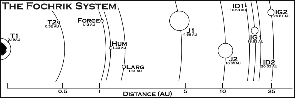
Today we build the calendar system for Hum, the humma homeworld in the Fochrik system, which we have been detailing in the previous posts (part 1, part 2) in this series.

The Data

image credit – JPL

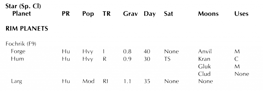
In the first part of this series, we established the following facts about Hum:

  • From Zebulon’s Guide to Frontier Space
    • Rotational period: 30 hours (we’re going to refine this a bit later on)
    • Surface gravity: 0.9g (which we increased the precision on to 0.91g)
    • 3 moons: Kran, Gluk, & Clud
  • From our calculations:
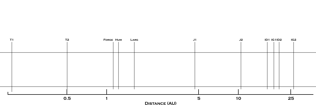
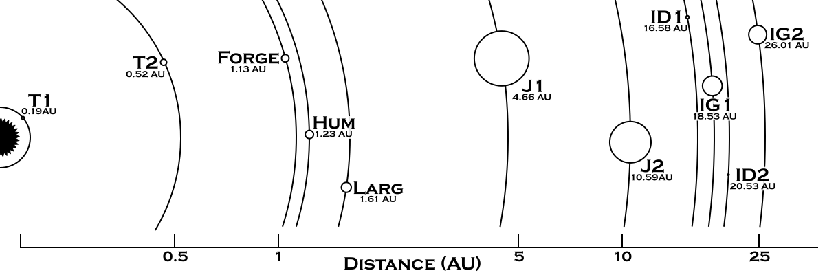
    • Orbital Distance: 1.23 AU
    • Orbital Period: 11323.3 hours
    • Density: 5.43 gm/cm3
    • Mass: 0.8139 Earth masses
    • Radius: 5,991.93 km

Of those parameters, we won’t be using the surface gravity, radius, or orbital distance in this analysis but we will be using the rest.

The Moons

I ignored the moons in the early parts of this series but now they become important so we need to detail them out a little bit more. Just as the orbital period of the Earth’s moon defines the concept of a month for us, given that this is the humma homeworld, the orbital periods of Hum’s moons would probably play a roll in defining their calendar system as well. So lets figure out the data on Hum’s moons.

All we really have to start with is the fact that there are three moons and their order (assuming the first one listed is the closest). Beyond that, we can really do whatever we want. That said, we have a few considerations to keep in mind.

First, Hum is smaller than Earth (about the size of Venus) and so has a smaller gravitational pull. This just means that the larger the moon, the more it will cause the planet to “wobble” about their common center of gravity. So we may not want any moon to be too big. It also means that if the moons have to be too far away, they might have escaped the planet’s gravity well. This latter point shouldn’t be an issue but is something to keep in mind.

Second, the moons will all mutually interact gravitationally. Which means if we have strong orbital resonances (orbital periods in small integer ratios), or if they have very close passes (with “close” depending on their relative sizes) as they orbit, the moon system may be unstable and not have survived to the present day.

So while we can pick anything we want, we should keep those ideas in mind. Now ideally, after picking the parameters for the moons and their orbits, I would generate orbital data for them all and run them through several hundred thousand or several million years of orbits to confirm stability but I didn’t do that. So we’ll just hope what we come up with something that makes sense and works.

The other thing to consider is what role we want to attribute to the moons in regards to the calendar system. This will have an impact on the orbital periods we pick.

Kran

From here on out we’ll be calculating time in hours and using the Galactic Standard Hour (which equals one Earth hour) as the value. In truth, there is no real reason for the humma to have an hour (or minutes or seconds for that matter) that correspond to that but it as useful measure to discuss the topic. There’s only so much new information you can wrap your mind about.

Kran is the innermost moon of the system. It will have the shortest orbital period of the three. As such, I decided that this moon would also be the smallest and associated with the “week” concept on Hum.

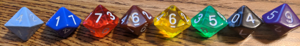
Since I want the “week” to be something on the order of 5 to 10 local days, and as I have no real reason to prefer one value of another, I’ll just roll 1d6+4 to get the value. I rolled a 5 so a Hum week is 9 local days long. Since the local day is 30 hours (from Zeb’s Guide), the week is 270 hours long. I want the orbital period of Kran to be something near this value so I just rolled four d10s to refine the number. The first one, I subtracted 5 from to get a number to add or subtract from 270, and the next 3 were just read as digits to represent the first 3 digits after the decimal place.

I rolled a 5 for the first die which meant no offset and then I got a 6, a 10(0), and a 4 so the orbital period of Kran is 270.604 hours. I realized later in the process that I should have probably given a bit more range the the +/- die but it’s fine as it is.

We’re also going to want to have a mass for the moon as that will have a small impact on its orbital distance. Since I wanted this moon to be small but still basically spherical, I just arbitrarily picked a size that was near to the size of the asteroid Ceres. I rolled some dice to pick exact values (although now I don’t remember exactly the rationale behind what I rolled) and came up with a value of 0.0125 times the mass of the Moon.

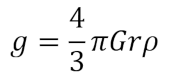
To get the size of the moon given its mass, we need its density. Referring back to the possible densities of the planets from the original article, I wanted to pick something in the 2-6 gm/cm3 range. So I rolled a d4+1 for the integer part and some d10s to get two decimal places and came up with
a density of 2.71 gm/cm3 for the moon.

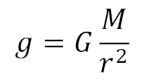
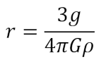
Okay, now we’re all set to calculate the final values. Determining the radius is straightforward, we’re just back to this equation:

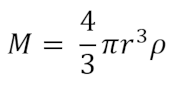
Only we’re solving for that r in there instead of M. That gives us a radius of 432.51 km. Next we want the orbital distance which takes us back to this equation:

where we are solving for a. M1 is the mass of the planet, and M2 is the mass of the moon. Again I used this handy website but since you can’t actually solve for a, I had to try various distances until I got the period to match. So it might have actually been faster to do the math on my calculator but oh well. We end up with a result of 198,336.5 km as the orbital distance for Kran.

For reference the diameter of Earth’s moon is 3474.2 km, almost exactly 8 times bigger, and it’s orbital distance is on average 384,400 km, so Kran is nearly twice as close.

Gluk & Clud

I’m not going to go over every detail of the other two moons but suffice it to say I followed the same procedure for each of those. The only constraints I had was that I wanted Gluk to be the largest of the three moons and have it’s orbital period correspond to between 1/8 to 1/14 of a year to represent the month concept. Clud was going to be way out there and orbit only about 4 times a year to correspond to the seasons.

After working through all the math we get the following results for each of the moons:

NameOrbital Period (hrs)Orbital Distance (km)Mass (moon)Density (gm/cm3)Radius (km)
Kran270.604198,336.50.01252.71432.5
Gluk1,026.836483,757.20.52373.141,430.2
Clud2,826.842948,883.70.24133.461,069.5

This image shows the sizes of the moons relative to each other and to Earth’s Moon. The image on the left shows their actual physical sizes if they were all side by side. The image on the right shows their apparent sizes as seen from the surface of Hum (assuming the Moon was dropped in at the proper distance).

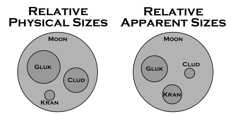
The moons are all physically smaller than the Earth’s moon by quite a bit and appear smaller in the sky. Also, notice that because Kran is so much closer than the other moons, although it is physically the smallest, it appears almost as big as Gluk and larger than Clud.

Hum’s Rotation Period

One more thing we need to establish is the actual rotation period of Hum. The information in Zeb’s Guide said it was 30 hours. However, I want to add a few more decimal places but still have it round to 30. So employing my usual method, I rolled d10-6 (to get a value between -5 and +4) and then two d10s for decimal places. I then added that to 30 to get the actual rotation period in hours. I ended up with 30.09 hours.

The Calendar

Now that we have all the physical data we need, we can get on to the actual purpose of this post, determining the calendar of the planet Hum.

Length of Year

The first thing to determine is the length of the year in local days. We have the orbital period of the planet (11,323.3 hours – about 30% longer than an earth year and 41.5% longer than the Frontiers’ Galactic Standard Year) and the rotation period of the planet (30.09 hours) so we just divide and find that the Hum year is 376.3144 local days long.

In local day terms, the year is only a bit longer than an Earth year, just 11 days more. It also tells us we’re going to need leap years, about every third year. We’ll come back to that.

In the previous sections, with the exception of the moon Kran, I sort of glossed over the relationship between the orbital periods of the moons as they relate to the length of the Hum year. Now let’s look at that in detail.

A Week on Hum

The inner moon Kran has an orbital period of 270.604 hours. Dividing this by the length of a day (30.09) hours, we get that Kran orbits every 8.993 days. That’s almost exactly 9 days. In fact, amazingly close to to exactly 9 days. Which is why I said above, I should have allowed for a bit more variation.

You might be suspicious of how well these orbital periods line up. The exact values selected were not completely arbitrary. I picked approximate values based on what I wanted to see and then let the dice tweak them slightly. And then I also manually tuned them a bit more. For example, I actually rolled 30.06 hours as the rotational period of the planet but when working out the leap years, liked the values I got for 30.09 hours better and went with that. So it’s no coincidence that the numbers come out so close. Maybe too close.

But that’s fine, sometimes you get lucky. So we’ll define a week on Hum to be 9 days long. At some point the start of first day of the week corresponds to the full Kran on the meridian but since the cycles slowly drift, that only occurs every once in a while and the phases slowly move through the week.

Comparing Kran’s orbital period to the year, we see that it makes 41.84 orbits each year so a typical year is almost 42 weeks long.

A Hum Month

If we compare the orbital period of the moon Gluk to the length of day we see that it’s orbital period corresponds to 34.125 days. And comparing it to the planet’s orbital period, it makes 11.02737 orbits in a single year.

Since I’m going to tie the concept of a month to the orbit of Gluck, a nominal month is 34 days long and there are 11 months in the year. There might be some variation like on Earth but this works as a base line.

With eleven 34-day months, that accounts for 374 of the 376.31 days of the year, leaving 2 extra days in the calendar. I’m going to assign one of those days to one of the months making it 35 days long (in the spring) and the other will be a holiday celebrating the passing/new year and will occur at the end of summer which will be when the Hum calendar year ends.

A Seasonal Moon

That leaves us with Clud. It’s orbit is 93.95 days long and it orbits 4.006 times each year, completing one orbit every season. Since the timing of its orbit doesn’t quite line up with the planet’s orbital period, the timing of the full phase of this moon slowly shifts (by just over half a day a year) over the centuries but the humma have tracked this for millennia and know the pattern.

Leap Years

All that’s left is to deal with that pesky 0.3144 days left over after each year. Multiplying by 3 gives us 0.943 days, which is just enough to be considered another day. Thus every third year, the end of year holiday is a two day event instead of a single day adding an extra day on that particular year but not part of any month.

It’s not quite a full day though and so every 51 years, the deviations add up enough that the extra day is not added to the calendar, just like on Earth when we don’t add in the leap day on years divisible by 100.

Finally, there is one more minor correction and that occurs every 1530 years. On that year, which would normally be a year the extra day is skipped, the extra day is included (just like including the leap day here on Earth in years that are divisible by 400 as occurred in the year 2000). This has only occurred once since this calendar was established and the next one won’t occur for another 172 years.

The Final Calendar

So the final Hum calendar looks like this:

  • One week is 9 days long – in modern times it is a 6 day work week with a 3 day weekend
  • Each year has 11 months plus one holiday at the end of the year to celebrate the harvest and ring in the new year. This feast day/beginning of the new year corresponds to the end of the Hum summer (what we would call fall)
  • One month consists of 34 days, or nearly 4 weeks. The exception to this is the 5th month which is 35 days long. This occurs during the planting season giving one more day in that month.
  • Every three years there is a leap day, extending the harvest holiday into a 2 day event instead of a single day.
  • Except that every 51 years, the leap day is skipped and every 1530 years the day that would be skipped is included.

One more thing we need is to anchor this calendar with the Frontier standard calendar. To do that I’m going to say that the start of Hum year 2898 will coincide with FY60.124 and that year is a leap year so the end of year celebration (that starts on FY61.290) will last two days.

Last Thoughts

I realized as I was typing this up, that I didn’t account for the difference between sidereal and synodic periods for the moons. The orbital periods listed are really the synodic periods (as seen from the surface of Hum) but I treated them like the sidereal periods for computing orbital distances. Which means the distances are a bit off. The differences would be relatively small but that’s something I should revisit in the future. The rotation period for Hum is definitely the solar period (noon to noon) and not the sidereal period.

Otherwise, this is a pretty good description of Hum and its moons and a reasonable calendar for the system. I didn’t touch on Forge or Larg, the two other inhabited worlds in the Fochrik system. I’m assuming this calendar predates the humma’s space age and so is the foundation of any other calendar system on the other worlds. How it was adapted might be another article in the future but for now is left as an exercise for the reader.

What do you think of the calendar system presented? What would you have done differently? What do you like? Let me know in the comments below.

March 19, 2019 Tom Leave a comment

How to Draw a System Map

Okay, in my last post on this topic, we generated all of the data needed to draw out a system map for the Fochrik star system. If you haven’t read the previous entry, you might want to but it’s not necessary. The next step is to take that data and turn it into the actual image. This post will cover that process. Let’s dive right in.

The Data

First a quick summary of the data for the system that we generated last time. While we won’t need all of this for the map, but it’s good to have it all summarized in one place. For generating the system map, we’re only going to need the orbital distance and the planet’s radius.

NameOrbital
Distance (AU)
Orbital
Period (hrs)
Gravity (g)Mass (Earth)Radius (km)
T10.19687.460.330.03492,064.55
T20.523,112.570.670.33734,468.50
Forge1.139,316.450.810.60125,443.75
Hum1.2311,323.30.910.81395,991.92
Larg1.6116,957.21.121.46227,215.22
J14.6683,501.43.30525.8279,714.14
J210.59286,0611.55140.1460,108.51
ID116.58560,3910.140.01892,297.74
IG118.53662,1060.9719.90228,62316
ID220.53772,1440.060.00181,054.47
IG126.011,101,0961.0218.47226,919.75

When drawing the map, we want the distances to be all on the same scale. However, we cannot use a simple linear scale in most cases as that would put all the inner planets right on top of each other if we want to see the outer planets on the same image. You can see this in the following diagram that has a linear distance scale.

Fochrik system planetary distances on a linear scale. Click for larger image.

As you can see, those inner planets are bunched up pretty close together while the outer planets have huge gaps. We want to spread out the inner planets while compressing the outer ones but still have the relative scale be correct. To do that we need to shift from a linear scale to a logarithmic one.

To get on a log scale, we are just going to take the base 10 logarithm (the ‘log’ key on your calculator) of each of the orbital distances and use that value to draw the distances. First I’ll present the numbers and then another simple drawing.

NameOrbital Distance (AU)Orbital Distance (log(AU))Scaled Distance
T1 0.19-0.721214
T2 0.52 -0.2840233
Forge 1.13 0.0531401
Hum 1.23 0.0899420
Larg 1.61 0.2087479
J1 4.66 0.6684709
J2 10.59 1.0249887
ID116.581.2196985
IG118.531.26791009
ID220.531.31241031
IG226.011.41511083

We can’t quite use the log(AU) values as the smaller numbers generate negative values (I’m not going to do a math lecture here. If you’re interested in why, you can check out this Wikipedia article). So we need to scale those numbers somehow. The scaled distance value in the table above was calculated by taking the log(AU) distances, adding 0.75 and then multiplying by 500. We’ll use these values to create the plot.

As you can see, the range of values is greatly compressed which allows things to be a bit more evenly spaced. The only issue with this scale is that zero (i.e. the position of the star) has a value of negative infinity so we’ll have to pick some arbitrary distance to separate them. However, since we’re just trying to show the relative position of the planets, that’s not too big of a problem. Here’s the simple plot we get:

Orbital distances on a log scale. Click for larger image.

This scale compresses the outer planets a bit but helps us spread out the inner planets which are the ones we’re more interested in anyway.

Drawing the Map

With the numbers above, we have all the information we need to create the map. The last thing to decide is if we are going do make a horizontal map (oriented like the diagrams above or the map in the Clarion Calendar post) or a vertical one (like in the Duergan’s Star post). For this map, I’m going to make a horizontal map simply because all of the “along the way” image will fit better into the post than a vertical one will. However, the process applies just as well to a vertical map, you just have to rotate everything 90 degrees.

I’ll be building the map in Inkscape, my vector drawing program of choice and it will be a simple black and white drawing so it shouldn’t be too complicated.

Here’s a video I made of the map building process if you want to watch it in real time, It’s about 53 and a half minutes long and completely unedited so you can see all my mistakes and fumbling around. If you don’t want to watch the video, I’ve described all the steps below.

Laying the ground work

To start, we want to set up the basic image and some guides for us to work with. I’ve decided to make the image 1200×400 pixels in size so I create a blank document of that size to work with. I also turn on a rectangular grid to help with position items. This grid will get turned on and off as needed during the drawing process.

I’m going to use the logarithmic distance scale for my planet spacing so I then import that image into my document and position it accordingly.

Finally, I draw a guide line down the middle of the image so I know where the center line is. After this initial setup, the image looks like:

I’ve shifted the imported image just slightly so that it’s 10 pixels to the right of where it was in the original. I wanted a little more space between the star and the first planet. Since I’ll be measuring the scaled distances from the left edge of the image, this means I’ll have to add 30 pixels to the values in the table above for the final radii of the orbits.

All of the above was done on the initial default layer. I then create three more layers: one for the orbits, one for the objects (star and planets), and a third for the labels. I like to work in lots of layers as it makes it easy to turn bits and pieces on and off and add in effects if needed.

The star and the orbits

The next step is to draw in the star itself and then start adding arcs for the orbits. The symbol for Fochrik is created using the star and polygon tool in the star setting with corners set to 30 and spoke ratio set to 0.8. This is drawn on the object layer.

Next I hide the objects layer and move to the orbits layer. Here I use the circle tool to draw in the first orbit. Clicking on the point where the center guide meets the edge of the image I then drag out the circle holding down the shift and the control keys until it reaches out to the position of the guide line for the planet T1.

Holding the control key down makes the circle drawn have integer ratios between the x and y directions allowing you get a proportional circle. Holding down the shift key makes your initial click point the center of the circle instead of the upper left corner of the box enclosing the circle. Once I have the circle drawn to approximately the correct size, I use the spinner boxes for Rx and Ry (the x and y radii) to set the exact radii (44 px in this case). The fill of the circle is set to transparent, the stoke is set to black with a thickness of 2 pixels.

Inkscape allows you to draw off the edge of the image so we drew a whole circle for this first orbit. Since we will be copying and scaling this up, we don’t want our circles going way off to the left. We can turn the full circle into an arc by grabbing the small circular mark on the drawn circle (it’s at the 3 o’clock position) and moving it clockwise to break the circle. I move it down to just past the 6 o’clock position. Then I go back and grab the other small circle node at 3 o’clock and move it up to just before the 12 o’clock position. This gives us a half circle which is all we need.

Now it’s just a matter of duplicating that arc and setting the correct radii for each one. As we move out we’ll want to adjust the size of the arc so it’s not sticking up well above or below the edge of the image just to make things a little cleaner on our drawing canvas.

We can duplicate a selected object by pressing Control-D. Then we just go up and set the Rx and Ry values based on the scaled distance values in the table above (remembering to add 30 to each one). You have to remember to have the circle tool selected while you do this or you can’t set the radii.

Once that is done, we have an image that looks something like this:

Notice how the arcs are going high. They will be cut off when we export the final image. They were originally also going low as well but they have been adjusted (at a later step) and I didn’t export an image while I was drawing them.

You might also notice that the arc for the planet T2 is not lined up with it’s guide line. That is because as I was drawing it, I noticed a discrepancy between where the guide line was and where the arc was drawn based on the scaled distance values. I originally though there was an error in the scaled distance but it turns out I just drew my guide sketch wrong. It’s always good to double check your work.

Drawing the planets

We’ve got our orbits, now we need to draw the planets. This will be done on the planet layer so we switch to that layer now.

Like the orbits, we want the planets to all be on the same scale. This obviously can’t be the same scale as the orbits or we wouldn’t be able to see them since they’d just be dots on the page. To pick the initial scale, I just let the radius of the circle we’re going to draw be equal to the radius of of the planet (in km) listed in the table divided by 2000. I computed each of these values and wrote them down on a piece of scratch paper to have them handy.

Depending on how you have Inkscape set up, when you draw in the first circle, you’ll notice that you just get an arc instead of a full circle. That was my case as I have Inkscape set to remember the last setting for the tool and use that instead of resetting to the default. I find that more useful. But we need to reset the tool to draw circles. This is done by finding the Start and End boxes (up by the Rx and Ry boxes) and setting them to 0 and 360 respectively. Now we’re drawing circles again. Also you’ll want to set the fill to white instead of transparent.

I then just move to an arbitrary point on each planet’s orbit, draw a small circle and then set Rx and Ry to be the values determined for that planet. It doesn’t matter exactly where you draw them as we’ll go back and properly position them once they are all drawn.

When you start doing this, you’ll quickly notice that the scale we’ve picked is simply too small for the small terrestrial planets. In the case of a few of them, you can’t even see the disk as it is smaller than thickness of the line we drew for the orbit. To solve this we simply double the radii of these planets. However, that would make the giant and Jovian planets too big if we doubled them as well. So we’re just going to have to have different scales. The terrestrial and ice dwarf planets will be to scale with each other as will the giant and Jovian planets but the smaller planets will be twice as big as they would be if they were to scale with the larger planets.

The last step of drawing the planets is to place them at an appropriate position on their orbit circle. There are two requirements here. One is that the disk of the planet should be centered on the orbit line. The other is that for planets with close orbits, they are spread out across the image so that when we add labels there won’t be any overlap. To make this easier you should turn off the grid that we set up at the beginning so the software isn’t trying to snap your circles to positions you don’t want.

Once that is done, we have an image that looks something like this:

You’ll notice that even doubling the scale, some of those planets are pretty tiny. In fact, you might not even be able to see ice dwarf 2 unless you click on the image above to get the full sized one. But that’s okay.

Adding labels

The next step is to label everything. There are a few things we want to put in our labels. The most obvious is the name of the planet. I still haven’t come up with official names for the planets but that doesn’t matter for the purposes of demonstrating the mapping technique. The other thing we need to do is add the scale for the system map. Finally we’ll add a label for the system. I’ll be using the Copperplate Gothic Bold font for my lettering.

Let’s start with the scale. If you watched the video, you’ll know that I actually did this way back at the beginning of the process. Since it was already there in the imported image, all I had to do was trace it. Once it was drawn in and had the numbers, I put the “Distance (AU)” label on and then moved everything down as close to the bottom of the image as I wanted it.

The labels on the the scale are drawn with a height of 16px for the numbers and 20px for the label. What you choose is arbitrary and it should be picked to match the size of the drawing. You don’t want it too small but you don’t want it too large either.

However, at this point, I didn’t like the orbit lines crossing over the scale and I went back and adjusted them so that they stopped just before touching it. If you look closely in the previous image, you’ll see another guide line that sits just above the scale that all the orbit lines touch. I drew this line in and then, using the circle tool, adjusted the end of the arc of each orbit line to just touch that line, which is why they don’t extend below the image.

Turning off the layer with the guides and the scale image gives us the following at this point. I’ve also now only exported the actual drawing so everything is trimmed appropriately.

Next we label the planets. For each planet I’m going to put the name in using a 20px high font and then centered under the name, put its orbital distance in a 10px high font. Again still using Copperplate Gothic Bold. I had originally intended to just type both and then change the font size of the distance but found that I couldn’t adjust the vertical spacing like I wanted to. So instead I created two text objects, one for each line, used the alignment tools to get them lined up, and then grouped the label for each planet into a single object so I can move it around easier later.

It doesn’t really matter exactly where you put the labels to begin with as you’ll be moving them around once they are done and you have their exact sizes. Just go through and add them for each planet. Then, once they are in the drawing, move and position them so that you like the placement. This may also involve moving the position of the planet’s disk on the orbit line to get a spacing you want.

Typically for the smaller planets, I like to place label so the center of name is aligned with the center of the disk. For the large planets, I tend to set it to the lower left or right corner depending on the exact positioning. I just do this by eye. You want to avoid having the text run over the orbit lines as much as you can but in some cases it’s unavoidable. Just place the names where it looks good to you. On a vertical map, I’ll often try to center the name of the planet under the planet’s disk.

Now we have to deal with the text that is overlapping the orbit lines. This often makes the text hard to read so we need to mask out the orbit lines under the text. Your text layer should be positioned above the orbit layer. If it isn’t you’ll need to move it up in the layer stack. What we’ll do is draw some white rectangles to hide the orbit line below the text. I like to set their opacity to about 75-80% so the orbit lines slightly peek through but you can make them fully opaque if you prefer. Drawing the rectangles can either be done on a new mask layer that is placed directly under the labels layer or in the labels layer itself.

In this image I drew the rectangles directly into the labels layer. Using the rectangle tool I just drew in a small rectangle over the orbit lines in each location there was overlap between the text and the lines. You’ll want to make the rectangle extend just a bit below and above the text. Exactly how much depends on how much space you want between the lines and the text and is a matter of taste. As you draw the rectangles, they are placed above the text so you need to send them to the bottom of the z-order for the layer so they are behind the text instead.

If you draw on a new mask layer, then you don’t have to worry about moving the z-order of the boxes as they will all be between the orbit lines and the text. You also don’t have to worry about the opacity on the individual boxes but can adjust the opacity of the entire layer all at once. This is typically how I do the masks but for some reason didn’t on this particular drawing. Probably due to the fact that I was recording and it slipped my mind.

We are almost done. At this point our image looks like this:

Finishing touches

The only thing left to add is the label for the system, a border, and a white background.

We’ll put the label in the upper left. We want this to be large so we’ll use a 32px high font. We’ll also need to add a mask as it will be overlapping the orbit lines. I considered simply adjusting the orbit lines to end below the label but decided to leave them in and mask them off.

The border and background I did with a single object. You may not have noticed, but all of the images so far have had a transparent background with just the objects drawn on it. This can cause some issues depending on how the image is rendered so we want to add a solid white background.

To do this I make a new background layer that sits at the very bottom of the layer stack. On this layer I draw a single large rectangle that stretches corner to corner across the entire image. I set the fill to white and the stroke to black with a 6px thickness. Due to the way Inkscape draws the stroke, half of that will be off the final image giving a 3px border. If you want it thicker or thinner, simply adjust the stroke width.

And now we’re done. Here’s the final image:

The final system map. Click for larger version

If you’d like to look at or play with the original SVG file of this map, they you can grab it here:

FochrikSystemMapDownload

Other touch-ups

Giving the planets some character

For this demo, I didn’t do anything special with the planets themselves. If you wanted to, you could add in cloud bands or rings on the giant planets to give them a little bit of character. Especially if they have features called out in their descriptions. I didn’t have any special descriptors so I left them as simple circles but that could be added in later.

The FTL Horizon

If I was doing this map for FrontierSpace, the other thing I would add in is a dashed arc at the position of the FTL Horizon, which in that game is the distance you need to be from the star in order to engage your Nova Drive to travel between the star systems. That would be an important bit of information for the map to include.

Asteroid belts

I also didn’t add in an asteroid belt in this system. If I did then I would determine the distances for the inner and outer boundaries of the belt and draw orbit circles on the guide layer at those distances. Then on the object layer I’d go in by hand and draw in all the asteroids. I work on a 2-in-1 laptop that has a stylus so I can actually flip my laptop into tablet mode and draw the asteroids with my stylus right on the screen. I find this much easier and faster than trying to do it with the mouse but it can be done that way (and I’ve done it that way in the past). There’s a bit more to it than that so I might do a mini article on drawing in asteroid belts.

Final thoughts

And that’s everything. I think the map turned out pretty well. I was actually surprised it only took a little less than an hour to draw it out once I had all the data. All told I probably spent about 2-2.5 hours creating the data and making the drawing. It would have taken a bit longer if I had had an asteroid belt to include or added details to the planets but that gives you an idea of the effort involved. It actually took me longer to do these two blog posts (5-6 hours total) than it took to actually do the work.

I still have one more post on the calendar system to do and that will come in March. I’d like to hear your comments, questions, or any suggestions you have about the process. What wasn’t clear? What would you like more information on? Did you try this yourself? If you did, share your results. Let me know below.

February 26, 2019 Tom Leave a comment

Building a Star System – Fochrik

In a couple of my timeline posts at the end of last week, I mentioned an annual competition on Hum in the Fochrik system, the homeworld of the Humma race in Star Frontiers. The tweets were as follows:

FY60.032 – Contestants, spectators, and reporters gather on Hum (Fochrik) for the annual Humma Jump Competition. Speculation is high that the current record in the standing long jump event of 38.272 meters will be surpassed this year. #SFTimeline

— Star Frontiers RPG (@StarFrontiers) February 7, 2019

FY60.034 – After two days of competition, Zonuul Usu of Larg (Fochrik) wins the Humma Jump Competition jumping 38.275m, beating the previous species record by 3 millimeters. Two others beat the previous record in the final round of competition but lost to Zonuul. #SFTimeline

— Star Frontiers RPG (@StarFrontiers) February 9, 2019

This immediately got me thinking about how the Hum calendar interacts with the Galactic Standard calendar of the Frontier and if the Rim had a different standard calendar.

Since in my Clarion calendar system post, I mentioned that I would probably do more calendar systems for other planets and in my last State of the Frontier post I said I would write about creating a system map, I thought I’d roll all of these thoughts and ideas into a series of “how to” posts as I flesh out the Fochrik system.

I’m planning on dividing this into three parts. In this first article, I’ll be talking about generating the astrophysical description of the system. We’ll go over what we know from published material, adding a bit to that, refining the details, and trying to generate a stable star system.

In the next post, I’ll actually walk you through the process of creating a system map for Fochrik like I did for the Duergan’s Star system.

In the third post, I’ll generate a calendar for the Fochrick system. I don’t know yet if all three planets will have a unique calendar or if Larg and Forge will base their calendar off of Hum’s. We’ll see when we get there. I’m not planning to address a standard Rim calendar at this time as I need to look over the other Rim systems first. That may be a future post.

Anyway, let’s get started.

What We Know

Let’s start with what we know from published materials, both original with TSR and material from the fan magazines. There isn’t much, but let’s assemble what we have.

The Rim was introduced in TSR’s Zebulon’s Guide to Frontier Space, vol 1 as the area of space that the three new races introduced came from. It was specifically left vague in the supplement. Whether they intended to flesh it out more in later volumes that never were published we’ll never know. On page 50, in the “Planets of the Frontier” table we have the following entry for Fochrik:

For this series of posts, we’re interested in the stellar spectral type (F9), the number of known planets (three in this case) and their rotational period (the Day column which is given in hours). Also, the number of moons might be used in making the system map and we should probably consider them in making the calendars as well. The other information is not needed for this endeavor.

Beyond that, there is little said about the system in Zeb’s Guide. The worlds of the Frontier have little blurbs with interesting facts about each of them but there is nothing on any of the Rim worlds. We’re basically left with a blank slate.

In a Star Frontiersman article (issue 15), entitled Humma Hop Back, TheWebtroll talked about the race but gave no information on the star system. Tom Verrault did a little bit of work on the Humma in issue 13 of the Frontier Explorer were he fleshed out their racial description some more but again nothing was really mentioned about their star system. However in another article in that same issue, where he adds detail to the boon’sheh, a fan created race from the early Star Frontiersman issues, he places them with the humma in the Fochrik system with the humma forcibly relocating the boon’sheh to Larg from their mutual homeworld of Hum. But that’s all we have.

In the end, we just have the table entry for the system to work with. Which tells us we have three habitable planets, some moons, and their approximate rotation periods. We get to create everything else so let’s dive in.

Fochrik

We start with the star. It is given a spectral type of F9. That makes it a little more massive and brighter than the sun but not by much. I like to use the table on this page for my starting point of stellar masses and radii as it has broken the data down in to details for each spectral classification. Plus the author has gone through, and based on the spectral energy distribution, given you the RGB colors for the star. I’m a little leery of the radius data on that page but we won’t be using that in this analysis.

From that page we get a mass of the F9 star for 1.1 solar masses. Looking at the adjacent spectral types, F9 and G0, they have listed masses of 1.2 and 1.1 respectively so that gives us a range to work with and tells us that the F9 star is probably a bit heavier than 1.1 solar masses but within rounding errors. Plus there is scatter based on other factors as well so we have some room to wiggle about. Let’s do some quick calculations.

The mass of the sun is 1.989 × 1030 kg. so we have a range of 1.1 to 1.2 times that to work with or from 2.1879 × 1030 to 2.3868 × 1030 kg. Like I did for White Light, I want a few more decimal places so I’m going to roll some dice for the digits. I’ll keep the 2 before the decimal place, roll a d4 for the first digit, and then d10s for everything else. That will possibly let me go slightly outside the range but that’s fine. Here’s what we get:

I ended up rolling a d8 and dividing by 2 just so it was easier to see in the picture. I just rolled the dice and then went left to right as they fell on my desk to pick the order.

So we end up with a stellar mass of 2.21766549 × 1030 kg which probably has more decimal places than we need but that’s fine.

Size of the Habitable Zone

The next thing we need to know is the range of the habitable zone for an F9 star. We’ve got to squeeze three planets into that area. We don’t need to be exact, but we want some reference. For this Wikipedia has a good article on the habitable zone that you can read to determine the various factors that go into determining it. There is also a really great picture (reproduced here) that almost gives us what we need.

The only real problem with this image is that the x-axis is in relative flux on the planet rather than distance. But I can work with that to get values for Fochrik.

We start by getting the percentages for the edges of the habitable zones. This is done by drawing a line across at the temperature of Fochrik (6140 K) and then drawing lines down from those to the x axis like this (the blue lines)

This gives us a range of 178% to 34% for the optimistic habitable zone and a range of 115% to 36% for the conservative one. Now we just need to turn those into distances.

The amount of starlight on the planet is dependent on three things. The first is the temperature of the star (which we’re taking to be 6140K. We could figure it out exactly based on the mass but that is a close enough approximation). The second is the radius of the star. These two give us the total luminosity of the star, L, which is proportional to R2T4. The final bit, which we are trying to solve for, is the distance from the star. The amount of starlight received at a planet, F (flux), is proportional to the luminosity of the star divided by the distance squared, i.e. F~L/D2.

Combining those gives us that the amount of starlight at a planet, F, is proportional to R2T4 / D2. or D ~ sqrt(R2T4 / F). If we work in ratios to the solar temperature, solar radius, measure distances in AU (the distance from the earth to the sun), and enter fluxes as multiples of the flux at the earth (i.e. flux at earth =1, 200% = 2, 50% = 0.5, etc), everything works out.

For this exercise, we’re going to assume the radius of the star is the same as the sun. In reality, it’s probably a little bit larger but we’re not going to worry about that. So we can drop the R2 term. The ratio of the temperatures is just 6140/5780 = 1.062283737. That raised to the 4th power is 1.273392. Plugging in those number gives the following distances for the four flux percentages:

  • 178% = 0.8458 AU (inner edge of optimistic habitable zone)
  • 115% = 1.0523 AU (inner edge of conservative habitable zone)
  • 36% = 1.8807 AU (outer edge of conservative habitable zone)
  • 34% = 1.9353 AU (outer edge of optimistic habitable zone)

Those numbers seem about right. The star is brighter and hotter than the Sun so it makes sense that the habitable zone is a little further out than in the solar system.

Placing the Planets

Now that we know where the habitable zone is, we need to place the planets and add other details to the system. We start with the three known planets, Forge, Hum, and Larg.

The Habitable Worlds

Each of these planets is habitable, with fairly large populations. As such, they need to be at least somewhere within the habitable zone. Also, since they are relatively low gravity worlds, around 1g, they should probably be close to or in the conservative habitable zone as the optimistic one is more for “super earths” which these are not.

Forge is the innermost world of the three and the name itself implies that it’s a hot world. I’m going to place it just inside the conservative zone. It’s livable, but its a bit on the warm side. We’ll place it at 1.08 AU from Fochrik.

Hum is the humma homeworld. As such we’d expect it to have a relatively nice, comfortable climate. If we go back to the flux calculation from above and find the distance for 100% we get a distance of 1.13 AU. That’s a little too close to the 1.08 AU I picked for Forge so I’m going to move it out just a bit further than that and place it at 1.23 AU. It will be a bit cooler than Earth receiving only 84% the amount of starlight.

Finally, we have Larg. This has the smallest population, medium instead of heavy, so I’m taking that to mean that it probably has a less hospitable climate (in addition to the higher gravity). Plus, if we’re using the fan material from the Frontier Explorer, it’s where the humma deported the boon’sheh to. We’ll place this one out towards the outer edge of the conservative habitable zone at 1.61 AU.

Now that our habitable planets have been placed we need to fill the rest of the system. There are a number of ways you could do this. I have a really old program called StarGen that makes solar systems around F, G, & K type stars based on habitability ideas presented in a paper by the Rand corporation. It works pretty well but doesn’t take into account modern information as that paper is from the 60’s or 70’s if I remember correctly.

You could also use the star system creation system presented in the FrontierSpace Referee’s handbook. It’s a good system as well. However, for this system I’m just going to be arbitrary. I’ll roll some dice for distances but beyond that, I’m just going to pick what I want in the system.

The Inner Worlds

Let’s start close. What is inside the habitable planets? I’m going to place two small worlds in there. They are small, hot, and airless. They probably have mineable mineral resources but they are not very hospitable. We’ll place these worlds at .19 AU and 0.52 AU from Fochrick. To get those distances I simply rolled 4d10 and 9d10 respectively and divided the number by 100 to get the AU.

The Outer Worlds

Next let’s move out from the inner system and see what’s out in the outer reaches. We’re going to add in 6 more worlds outside the habitable zone. For now, I’m not planning on having an asteroid belt but that may change when we do some sanity checks below. We’re going to add the following planets to the system:

The truth is, it probably doesn’t matter how you generate the planets, their types and masses, and their distances. As long as you don’t repeat the same patterns over and over. The universe is vast and as modern exoplanet discoveries have shown, you can get all kinds of crazy systems. As a general rule, I allow anything to happen. Once. The more off the wall the idea is, the less likely I am to allow it to enter the setting twice but anything is possible once.

  • Jovian – 4.66 AU
  • Jovian – 10.59 AU
  • Ice dwarf – 16.58 AU
  • Ice giant – 18.13 AU
  • Ice dwarf – 20.53 AU
  • Ice giant – 26.01 AU

In each of these cases, to get the distance I created a number between 1 and 6.99 by rolling a d6 and two d10s. The d6 was the integer bit and the two d10s were the decimal bit. I then added that number on to the orbital distance of the previous planet. Like I said, this was going to be pretty arbitrary. Let’s keep going.

Orbital Periods

Now that the planets are all placed, we want to compute their orbital periods to know how long the length of their orbit is. While we don’t need this to create the map of the system. We want to do some sanity checks since the planetary placements were fairly arbitrary.

Orbital periods are given by Newton’s form of Kepler’s Third Law of Planetary motion, namely:

which I described in the Clarion Calendar post but P is the orbital period, a is the distance from the star, G is the gravitational constant, and M1 and M2 are the mass of the star and planet respectively. Since M1 >> M2, we’ll ignore M2 in our calculations.

You could do this by hand, or use a spreadsheet, or use an on-line calculator. I’m going to use this handy website that allows you to enter the values in a number of different units and does the math for you. I’m just going to leave the mass of the planet at 1 earth mass in the calculation. If I was going for full detail, I’d figure out the mass of each of the planets but this is really just an approximate sanity check. For example, if I set the mass of the first Jovian planet to 100 earth masses, it would lengthen the orbital period by only 10 hours, so it’s not something I’m going to worry about here.

Plugging in the values for the planetary orbital distance and the mass of the star we get the following data:

PlanetOrbital Distance (AU) Orbital Period (hours)
T10.19687.46
T20.523112.57
Forge1.139316.45
Hum1.2311323.3
Larg1.6116957.2
J14.6683501.4
J210.59286061
ID116.58560391
IG118.53662106
ID220.53772144
IG126.011101096

Planetary Names

I should really come up with names for the other planets but since this is the humma homeworld, the names should tie into their history and culture and I haven’t really thought too much about that yet. I’ll leave naming for a future post or as an exercise for the reader.

Mainly here I’m just looking to see that we don’t have any resonant periods with the two Jovian planets. With orbital periods in ratios such as 2:1, 3:2, & 3:1 we would have potential stability issues. My only concern is with the second jovian and the first ice dwarf. They are in a nearly 2:1 orbital resonance but that might actually be okay and why that planet is where it is. So I’m going to leave it alone. If I really wanted to check system stability, I’d generate the masses, starting positions and velocities, and then enter all of that into a simple n-body computer simulation and run it for a million years or so of simulated time to make sure nothing went crazy but I think this will be fine.

Planetary Sizes

Okay, while this isn’t strictly necessary to draw the system map, we might as well figure out how big each of the planets are (and their surface gravity. When I do the system map, I like to have both the distances to scale and the sizes of the planets to scale so if I want to do that, I need the sizes.

The equation we’ll be using for this is

where g is the acceleration due to gravity (m/s2), M is the mass of the planet (kg), r is the radius of the planet (m), and G is just the gravitational constant (6.67408 × 10⁻¹¹ m3 kg-1 s-2). Additionally we’ll want an equation relating the mass of the planet to its density which is just the volume of the sphere times the density or

where ρ is the density (kg/m3). While we could do this just with the mass, I like to make sure the physics work out for the type of planet so I like the densities to make sense and prefer to include it in the calculations. Combining those two equations gives us an equation that relates the gravity, the radius, and the density:

This is what we’ll be using to get the data we need.

Densities

As part of this we’ll need densities for the planets. We’ll just be picking those from reasonable ranges which are the following (in g/cm3):

  • Terrestrial (rocky) Planets – 3.5 – 5.7
  • Ice Dwarfs – 1.8 – 2.5
  • Ice Giants – 1.2 – 1.8
  • Jovians – 0.6 – 1.4+

To get it into the units we need (kg/m3 ) we just multiply by 1000. The Jovian planets may not have an upper density limit because once you get to be the size of Jupiter, adding more mass doesn’t change the radius much, it just increases the densities. Brown Dwarfs, which are 10-80 times Jupiter’s mass are still all about the same size.

We’ll use these density ranges to pick densities for the individual planets in the sections below.

The Habitable Planets

First up are the three habitable planets that we know the gravity on. In this case we need to rearrange the last equation to solve for r giving us:

A Note on Gravity

For Star Frontiers, I’ve adopted the conventions that 1g = 10 m/s2 rather than 9.8 m/s2 as on Earth.  It makes all the math in the end easier and there isn’t much difference.  I figure that if you have all the races coming from different worlds, it would make sense that they standardized on a round number instead of some arbitrary fraction.

All that’s left is to pick a density or each of the planets and start computing. Well, almost. I also want one more decimal place for the actual gravity of the planet. To get that I’ll roll d8-4 x 0.01 and add that to listed gravity to give me some variation that would round to the listed value.

The table below is what we ended up with. Interestingly, all the gravity adjustments I rolled were positive. I also selected the planets with the higher gravity to be a little more dense but modulated that somewhat due to the fact that planets that form closer to the star would have higher density as well. Thus the densities of these three planets are pretty close together.

NameGravity (g)Density (gm/cm3) Mass (Earth)Radius (km)
Forge0.815.320.60125,443.75
Hum0.915.430.81395,991.93
Larg1.125.551.46227,215.22

Hum turns out to be almost exactly the same size and mass as Venus, just a little further out in the system so it’s not as hot. Forge is smaller still by about 10% in radius and 75% in mass while Larg is about 13% larger in radius than the earth and almost 50% more massive.

Other Planets

Now lets due the rest of the planets in the system. In this case we have to pick two of the three values: radius, density (or mass), and surface gravity. I’m going to select the radius and density for each of these planets and then compute the mass and surface gravity. Surface gravity doesn’t exactly make sense for the giant planets (jovians and ice giants) but it is the gravity present if you were stopped at that radius at it’s upper atmosphere. Here’s the table:

Name Gravity (g)Density (gm/cm3)Mass (Earth)Radius (km)
T10.335.650.03492,064.55
T20.675.390.33734,468.50
J13.301.48525.8279,714.14
J21.550.92140.1460,108.51
ID10.142.220.01892,297.74
IG10.971.2119.90228,623.16
ID20.062.190.00181054.47
IG21.021.3518.47226,919.75

J1 is almost two times the mass of Jupiter while IG2 is a little smaller than Pluto. If you want to compare them exactly this Planetary Fact Sheet page gives the data for all the planets in the solar system.

Wrapping up for now

And that’s it for this entry. We have the number of planets in the system, mass data on the star, and orbital and size data on the planets. I’m fairly confident that we don’t have to worry about system stability issues (of course since I didn’t do a rigorous check, this will be the one time it doesn’t work 🙂 ).

In the next post, we’ll create a system map for Fochrik and walk through the process of doing so. If you have any questions or comments, let me know below.

February 12, 2019 Tom 3 Comments
Become a Patron!

Recent Posts

  • Detailed Frontier Timeline – FY62.069 to FY62.99
  • State of the Frontier – August 2022
  • Battle of Hargut (Gruna Garu) – FY62.098
  • Archived Arcane Game Lore Posts – May 2013 to Dec 2014
  • A Look at Yachts and Privateers
  • Homeworld Bound – A Campaign Concept
  • Second Battle of Fromeltar (Terledrom) – FY62.083
  • Sample Star System Data
  • Detailed Frontier Timeline – FY62.038 to FY62.068
  • State of the Frontier – July 2022

Categories

  • 3D Models
  • Adventures
  • Background
  • Creatures/Races
  • Deck Plans
  • Equipment
  • Game Design
  • General
  • Locations
  • Maps
  • NPCs
  • Optional Rules
  • Patreon-only
  • Project Overviews
  • Reviews
  • Setting Material
  • Starships
  • System Brief
  • Vehicles
  • Writing

Recent Comments

  • Loguar on Detailed Frontier Timeline – FY62.069 to FY62.99
  • Loguar on Detailed Frontier Timeline – FY62.069 to FY62.99
  • Tom on Detailed Frontier Timeline – FY62.069 to FY62.99
  • Rook on Maps and Counters
  • Loguar on Detailed Frontier Timeline – FY62.069 to FY62.99
  • Tom on Detailed Frontier Timeline – FY62.069 to FY62.99
  • Tom on Second Battle of Fromeltar (Terledrom) – FY62.083
  • Loguar on Detailed Frontier Timeline – FY62.069 to FY62.99
  • Loguar on Second Battle of Fromeltar (Terledrom) – FY62.083
  • Aemon Aylward on Sample Star System Data

Archives

  • September 2022 (1)
  • August 2022 (9)
  • July 2022 (3)
  • June 2022 (3)
  • May 2022 (3)
  • June 2021 (1)
  • April 2021 (1)
  • February 2021 (4)
  • January 2021 (6)
  • December 2020 (5)
  • November 2020 (11)
  • October 2020 (4)
  • September 2020 (5)
  • August 2020 (4)
  • July 2020 (6)
  • June 2020 (5)
  • May 2020 (8)
  • April 2020 (5)
  • March 2020 (5)
  • February 2020 (5)
  • January 2020 (5)
  • December 2019 (7)
  • November 2019 (4)
  • October 2019 (6)
  • September 2019 (5)
  • August 2019 (6)
  • July 2019 (7)
  • June 2019 (5)
  • May 2019 (6)
  • April 2019 (7)
  • March 2019 (4)
  • February 2019 (5)
  • January 2019 (7)
  • December 2018 (5)
  • November 2018 (10)
  • October 2018 (4)
  • September 2018 (4)
  • August 2018 (5)
  • July 2018 (4)
  • June 2018 (4)
  • May 2018 (12)
  • December 2015 (1)
  • November 2015 (2)
  • December 2014 (4)
  • November 2014 (3)
  • June 2014 (1)
  • January 2014 (1)
  • July 2013 (1)
  • June 2013 (2)
  • May 2013 (3)

Meta

  • Log in
  • Entries feed
  • Comments feed
  • WordPress.org
Powered by WordPress | theme Layout Builder